Though we’re obviously huge Power BI fans here at Seer, we still hold a lot of love for Google Sheets as a way to quickly clean up and manipulate data as well as a way to clearly present a lot of our deliverables to our clients.
While Vlookups and Pivot Tables get most of the hype, there are a lot of useful functions and tips that don’t get a ton of visibility out there. Here are 3 you might want to add to your G Sheets toolbox.
1.Import XML
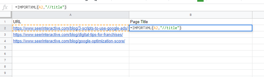
One of the first hot Google Sheets tips I learned after joining Seer was Import XML. This handy function enables you to pull in all kinds of data directly from a URL.
Syntax: =IMPORTXML(URL, “Xpath of the element you want”)
For example, if you wanted to pull in a title tag for a specific page, you would use:
=IMPORTXML(URL, “//title”)
This extends to any Xpath you find on a page. Here are some common ones that are useful for SEO practitioners:
- Title Tag: “//title”
- Extract meta description: "//meta[@name='description']/@content"
- H1: "//h1"
 2. Translate
A relatively new addition to the G Sheets, the translate function allows you to translate words into other languages. While the translations should always be checked for accuracy by a native speaker, this can be useful for quick translation of a list of keywords or a meta description.
Syntax: =TRANSLATE(“string”, “source language”, “translated language”)
In addition to the text you want to translate, you’ll need to enter the two-letter language code for both the source language and the language you want to translate your text into. Alternatively for your source language, you could enter “auto” and let Google automatically detect the language.
3. De-Dupe Your Data
It took a long time, but in early 2019 Google Sheets finally caught up with Excel and started enabling users to identify and remove duplicates from sets of data. To do this:
- Select the range of data you want to remove duplicates from
- Navigate to the Google Sheets menu > Data > Remove Duplicates
- You’ll then get a pop-up asking to confirm the columns you’re looking for duplicates in, hit “OK” and…
- That’s it! You should get another pop-up letting you know exactly how many duplicate values were removed from your range of cells
Similarly, you can also create a list of unique values from a range of data that you know contains duplicates with the Unique function.
Syntax: =UNIQUE(Data Range)
That’s it! If you have any favorite formulas in Google Sheets, let us know in the comments below.
If you’re interested in getting more tips directly to your inbox, sign up for our newsletter!

.png)